In (counterfactual) Treatment Effects Analysis, we learn that a fundamental condition in order to be able to estimate treatment effects reliably is that the treatment variable is “ignorable conditional on the control variables” (see Rosenbaum and Rubin 1983). When ignorability does not hold, as it happens with most cases of observational, non-randomized data, various methods have been developed to obtain ignorability, or in more precise words, to construct a sample (through “risk adjustment”, “balancing on propensity scores”, etc) that “imitates” a randomized one.
We are also told that ignorability is analogous to regressor exogeneity in the linear regression setup, and so that when ignorability does not hold, essentially we have endogeneity and the estimation will produce inconsistent and so unreliable estimates, see e.g. Imbens (2004), or Guo and Fraser “Propensity Score Anaysis” (2010), 1st ed., pp 30-35.
This is simply wrong. The treatment variable may not be ignorable and yet the estimator can be consistent. This means that we can estimate consistently the treatment effect even if the treatment is non-ignorable. We illustrate that non-ignorability does not necessarily imply inconsistency of the estimator, through the widely used Binary Logistic Regression model (BLR).
The BLR model starts properly with a latent-variable regression, usually linear,

Where  is the unobservable (latent) variable,
  is the treatment variable,
  is the vector of controls and
  is the error term. We obtain the BLR model if we assume that the error term follows the standard Logistic distribution conditional on the regressors,
  . Then we define the indicator variable
 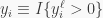 , which is observable, and we wonder what is the probability distribution of
  conditional on the regressors. We obtain

and in general,
![\Pr\left (y_i | \{T_i, \mathbf z_i\}\right) = \left[\Lambda\left (\beta_0 + \beta_1T_i + \mathbf z'_i \gamma\right)\right]^{y_i}\cdot \left[1-\Lambda\left (\beta_0 + \beta_1T_i + \mathbf z'_i \gamma\right)\right]^{1-y_i}\;\;\;\;(3)](https://s0.wp.com/latex.php?latex=%5CPr%5Cleft+%28y_i%C2%A0+%7C+%5C%7BT_i%2C+%5Cmathbf+z_i%5C%7D%5Cright%29+%3D+%5Cleft%5B%5CLambda%5Cleft+%28%5Cbeta_0+%2B+%5Cbeta_1T_i+%2B+%5Cmathbf+z%27_i+%5Cgamma%5Cright%29%5Cright%5D%5E%7By_i%7D%5Ccdot+%5Cleft%5B1-%5CLambda%5Cleft+%28%5Cbeta_0+%2B+%5Cbeta_1T_i+%2B+%5Cmathbf+z%27_i+%5Cgamma%5Cright%29%5Cright%5D%5E%7B1-y_i%7D%5C%3B%5C%3B%5C%3B%5C%3B%283%29&bg=f9f9f9&fg=333333&s=0&c=20201002)
This likelihood is estimated by the maximum likelihood estimator (MLE).
Turning to ignorability, it can be expressed as

Essentially ignorability means that the treatment variable is totally determined by the controls, or maybe, that if it is only partly determined by them, its other “part” is independent from the dependent variable/outcome.
Comparing  with
with  we see that ignorability of treatment in the context of the BLR model, is equivalent to the assumption
  .
.
“Great”, you could say. “So run the model and let the data decide whether ignorability holds or not”. Well, the issue is whether, when ignorability does not hold, the MLE remains a consistent estimator so that we can have confidence in the estimates that we will obtain. And the assertion that we find in the literature, is that non-ignorability destroys consistency.
Does it? Let’s see: in order for the MLE to be inconsistent, it must be the case that the regressors in the latent-variabe regression (eq. 1), are correlated with the error term. The controls are assumed independent from the error term from the outset. What is argued, is that if is non-ignorable, then it is associated with .
We just have seen that ignorability implies that  . So if non-ignorability is the case, we have that
  . How does this imply the inconsistency condition “ is not independent from “?
It doesn’t. The (informal) argument is that if the treatment variable is not fully determined by the controls, it “must” be statistically associated with the unmodeled/random factors represented by . But there is nothing here to support a priori this assertion. Whether the treatment variable is endogenous or not, must be argued per case, with respect to the actual situation that we analyze and model. Certainly, if the argument is that the treatment is ignorable, then, if the controls are exogenous to the error term (which is the maintained assumption), so will be the treatment variable also. But if it is non-ignorable, it does not follow automatically that it is endogenous.
Therefore, depending on the real-world phenomenon under study and the available sample, we may very well have a consistent MLE in the BLR model, and so
a) be able to test validly the ignorability assumption, and
b) estimate treatment effects reliably even if the treatment is non-ignorable.–
ADDENDUM
At the request of a comment, here is a quick Gretl code to simulate a situation where the Treatment is not ignorable, but it is independent from the error term and so it can be consistently estimated. Play around with the sample size (now  ) , or embed the script into a simple index loop (with matrices to hold the estimates for each run, then fill a series with the estimates from the matrix, then take basic statistics to see that the estimator is consistent).
<hansl>
nulldata 5000
set hc_version 2 #uses HC2 robust standard errors
#Data generation
genr U1 = randgen(U,0,1) #auxialiary variable
genr Er = -log((1-U1)/U1) #Logistic error term Λ(0,1)
genr X1 = randgen(G,1,2) # continuous regressor following Exponential
genr N1 = randgen (N,0,1) # codetermines the assignment of treatment
genr T = (X1+N1 >0) #Bernoulli treatment
genr yL = -0.5 + 0.5*T + X1 + Er # latent dependent variable
#The Treatment is not ignorable because it influences directly the latent dependent variable.
genr Depvar = (yL >0) #obseravble dependent variable
#Estimation
list Reglist = const T X1 #OLS estimation for starting values
ols Depvar Reglist –quiet
matrix bcoeff = $coeff #starting value scale parameter of the error term
#This so that the names of the variables appear in the estimation output
string varblnames = varname(Reglist)
string allcoefnames = varblnames
#command for maximum likelihood estimation
catch mle logl = Depvar*log(CDF) + (1-Depvar)*log(1-CDF)
series g = lincomb(Reglist,bcoeff)
series CDF = 1/(1+ exp(-g)) #correct specification of the distribution of the error term
params bcoeff
param_names allcoefnames
end mle –hessian
</hansl>


 ?
? and
and  have Normal marginals and they are independent, then they are also jointly Normal. By the Cramér-Wold theorem, it then follows that all linear combinations of them (like their sum, difference, etc) are also marginally Normal. If we want to consider more than two random variables, then for the above to hold, they must be jointly independent, and not only pair-wise independent. If they are only pair-wise independent, then they may be jointly Normal, may be not.